PART 7: MEASURING MOVEMENT IN LIVE CELLS
When we capture cells over time, also known as times series or live cell imaging, we are presented with more analysis options. along with the other types of analysis presented above, we can also get several pieces of information from time series by tracking objects over time or exmining the dynamics of the cells or their organelles.
In this section we will show you two different methods for tracking objects in time series, as well as how to present the dynamics of a cellular component in a single imge (known as a kymograph). We will use the images MovieStack.tif, AutoTrack.tif and Kymograph.tif for demonstration.
Manual Tracking
The simple method for tracking objects over time is to manually track them using the Manual Tracking tool.
Open the time series MovieStack.tif and then open the Manual Tracking tool from the menu Plugins -> Tracking.
![]()
In the Tracking window, tick on Show Parameters? to see and set all calibration settings. You can then set your parameters, including Time Interval (5mins for this example). If the xy calibration (scale) is not set automatically, enter the calibration value too (in this example it is automatically set correctly).
Select the option to show the tracks on the image if required by checking the box next to Show path?
![]()
When you have set your parameters, click Add Track to start your first track.
![]()
Then to begin tracking, click on the image in the centre of the object you want to track. The series will automatically move to the next frame. Click the centre of the object again.
Continue until you have reached the end of the series. If you have selected an option to show the track it will be visible overlayed in the image as a segmented line. Measurements for the object will be displayed in a results table.
Measurements will be displayed separately for each time point, these can be exported to excel and averaged.
Note 1: Manual tracking results are cumulative. You can check the "track number" column in the results to see which results belong to which track, or save and then clear results between each cell or each image to ensure you know which results belong to which cell.
Note 2: The first measurements will not be accurate as the object had not moved yet (ie: first measurement for distance is -1) and these should be removed from the data before averaging, and is not considered manipulation of data as it is not an actual measurement.
![]()
Repeat the process above (from Add track) for each cell you want to track in the image. Generally we would avoid tracking cells that divide, leave or enter the field of view. If cells cross paths, make sure you are able to determine which cell is which once they separate again, otherwise exclude these from tracking as well.
If you make a mistake during tracking you can Delete the last point (1 below) or select the track number from the drop down list and click on Delete track (2 below) to remove it entirely and sart again.
![]()
TrackMate: Automated Live Cell Tracking
For large numbers of cells, very fast movment or long imaging times it can be difficult to track cells manually. For these circumstacnes you can do automated tracking.
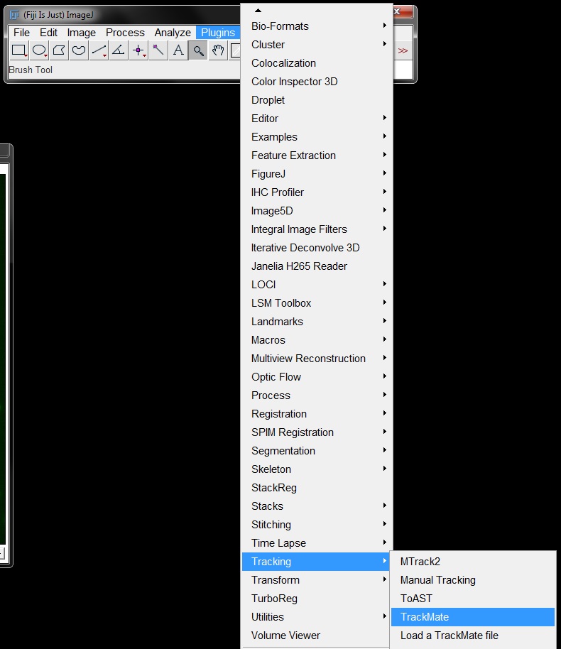
First open _AutoTrack.tif _in Fiji, then go to Plugins -> Tracking -> TrackMate.
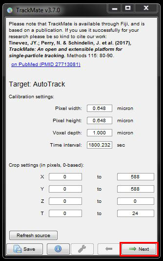
In the first window, you can set the scale of your image (should be pre-filled if your image is scaled). you can also add a region of interest here if you only want to analyse part of your image. As our image is scaled correctly and we want to analyse the whole image we don't need to make any changes here. Click Next to continue.
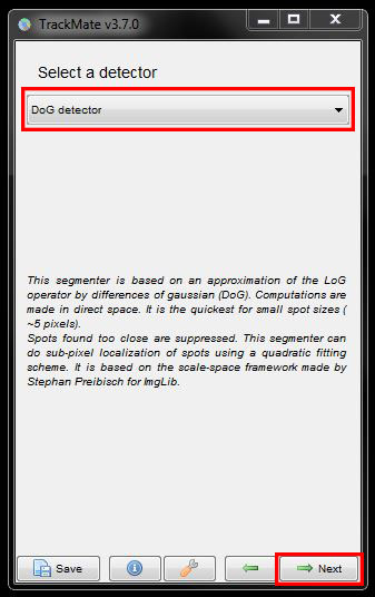
There’s different methods of detecting cells, the most common ones are LoG (Laplacian of Gaussian) and DoG (Difference of Gaussian). For this image choose DoG detector from the drop down menu the click Next.
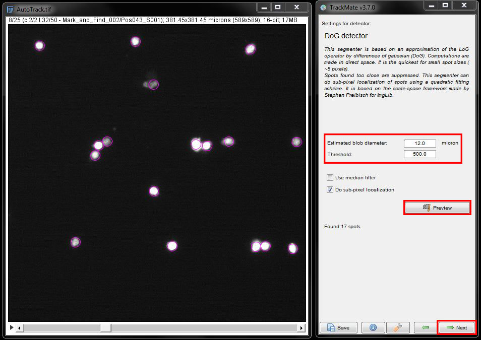
In the next window, enter the expected size of your cells and a threshold. Here, please enter a diameter of 12 microns for cell size and threshold of 500. Click on Preview to see what it detects. Repeat this at several different time points and adjust the diameter and threshold if needed to better detect the cells and eliminate any background signal that gets detected. When you are happy with your selection click Next to continue.
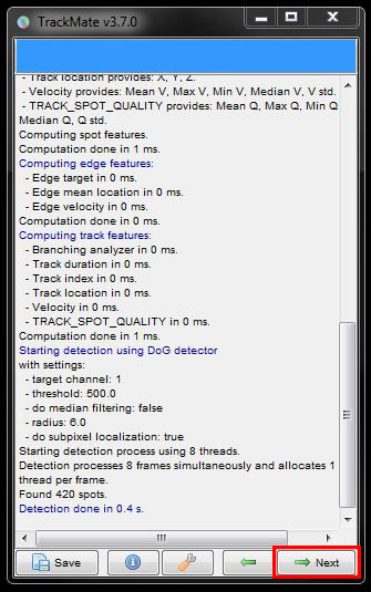
The TrackMate plugin will analyse each image in the time series and detect all cells with the given parameters. Once the detection is finished, press Next again.
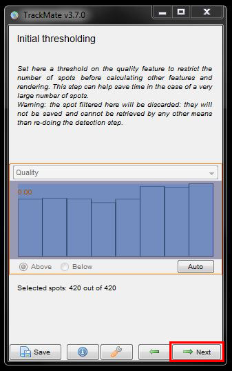
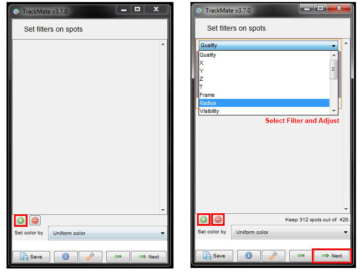
Now there’s options to filter out cells according to their quality. You can adjust the filter threshold using the sliders or try the Auto threshold settings by clicking on the Auto button. For this data set though, we’ll ignore this filter and press Next.
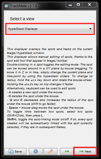
The next window will ask you to chose the view mode from a drop down menu. Here we will leave it as Hyperstack and again click Next to continue.
Another set of filter options will come up. To add a filter, click on the green plus button then select the filter from the drop down menu and adjust the corresponding threshold. You can add several filters by repeating this process for each. For this data set, we’re again going to ignore these filters. So remove any filters you have added, by pressing the red minus button, and then click Next.
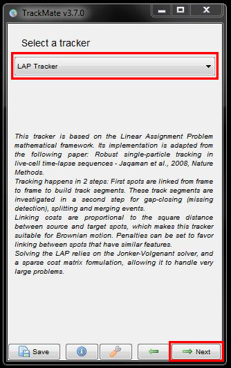
This brings us to the tracking options. All the options are different algorithms on how to connect the detected spots. Descriptions of the algorithm and how they work are given below the selected algorithm. Simple LAP Tracker will work well in most cases but here, we want to use specific parameters and penalties, so we need to choose the LAP Tracker (LAP = Linear Assignment Problem). Select this option from the drop down menu then click Next to continue.
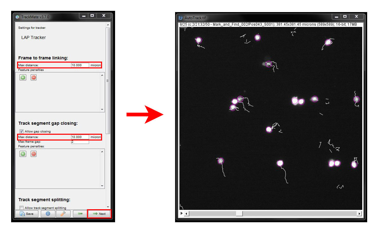
In the next window, you can set distances on how far you expect your cells to travel per frame. Set your distances for Frame to frame linking and Gap closing and click Next to assess the tracking accuracy.
We can try a few different settings here to see what best fits our data:
Under Frame to frame linking set the Max Distance as 10 microns and under Gap closing again set 10 microns.
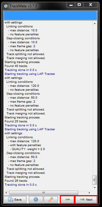
 At any point here you can click the Back arrow after tracking (in the log window) to return and change the parameters or Next (in the log window) to keep the tracks and continue.
Our initial settings didn't track our cells very well. You can see that some tracks are broken up into several tracks as the cells moved more than 10um between frames and some cells are not tracked for the entire time series. So lets try some different settings:
Under Frame to frame linking set the Max Distance as 120 microns and under Gap closing again set 50 microns.
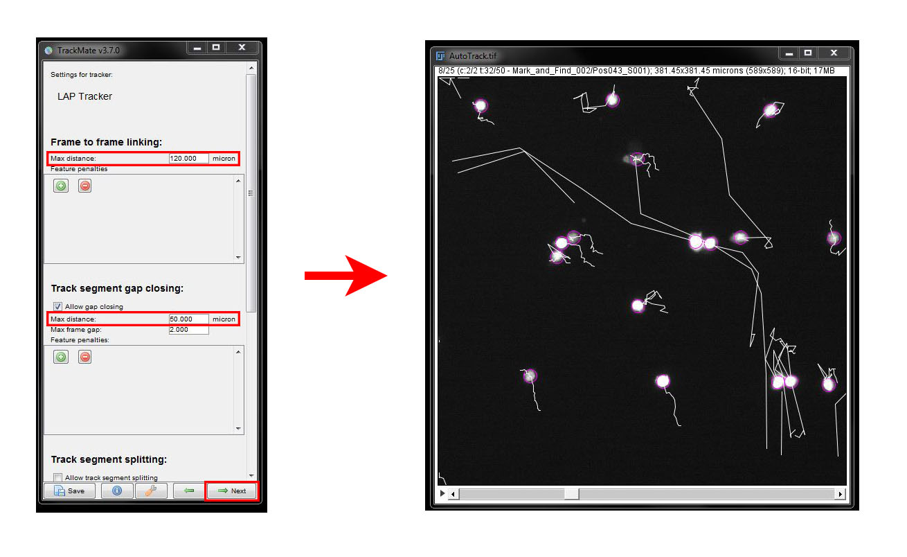
Here we see that the tracks are now better connected. Scroll thorugh the time series a few times and look for any errors in the tracking.
We do have a couple of cells that are not being tracked accurately. To ammend this we will use Feature Penalties. Go back to the tracker settings using the Back arrow button. Under Frame to frame linking click the green plus button. From the new drop down menu select the Quality filter and adjust the threshold for the filter to 2. Click Next to see the result.
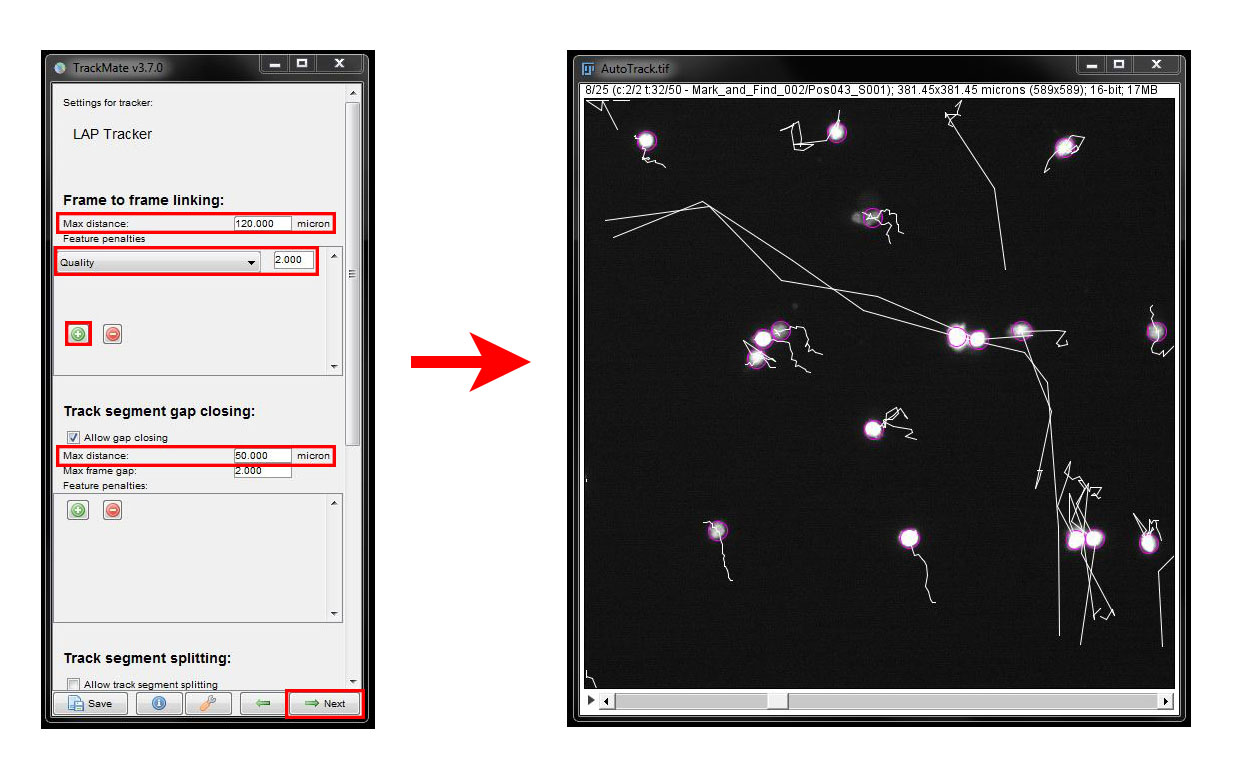 The two long tracks in the centre of the field of view are now a more accurate respresentation. As always, you will have to find the right settings for your data each time you use an analysis tool. When you are happy with your tracks, click Next in the log window to continue.
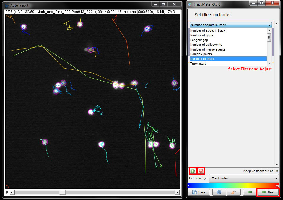
In the next step you will find Filter tracks, similar to the spot selection filters before. To add a track filter, follow the same protocol as spot filters; press on the green plus button, choose your filter from the drop down menu and adjust the threshold. Repeat for any additional filters you want to add. I am not going to use any additional track filters on this data, so use the red minus button to delete any you have added, then click on Next.
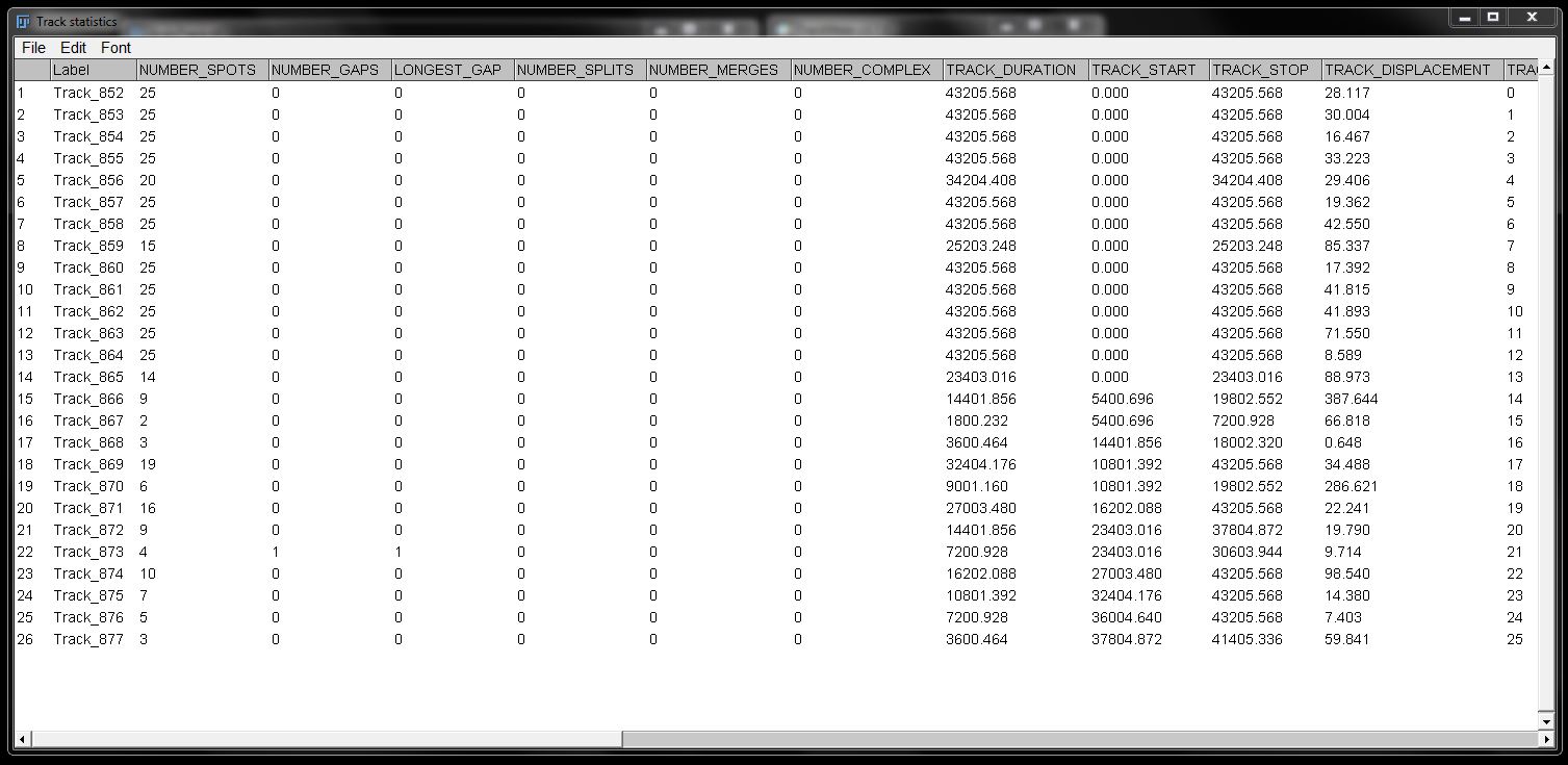
Now we can export the results of our analysis. In this window click on the Analysis button.
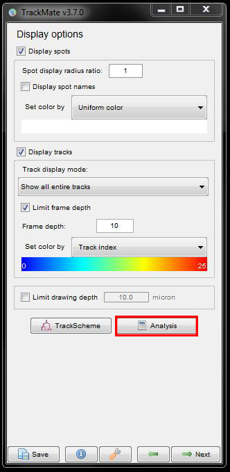
This will open tables with all the information on all your detected tracks and spots. You can save these as .csv and open in Excel or Prism for further analysis. The summary of the results is best found in the Track Statistics window. We have 26 tracks listed with results such as duration, displacement, and speed.
Kymographs
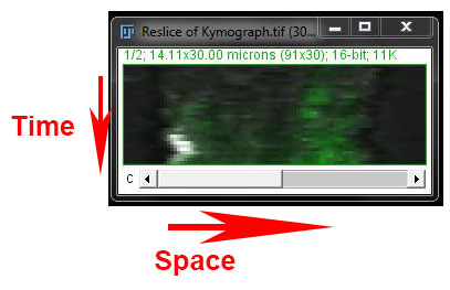
Kymographs are a way to represent a dynamic process as a single image. They are particularly useful to monitor and characterize the movement of a cell, membrane or organelle or a change in fluorescence over time. They can be seen as an x-t scan, where the intensity along a given line is plotted for all images of a time series. Each time point gives an intensity line, plotted e.g. along the x axis of the kymograph. These lines are stacked along the y axis for all frames. So we get an image where we move through space in the x direction and time in the y direction.
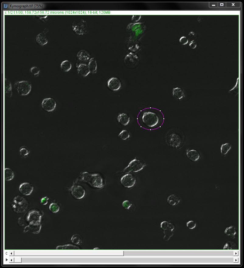
Open Kymograph.tif and scroll through time to find a cell that stays in the same area for the whole time series. An example of one of these cells is shown inside the ROI below.
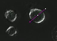
Switch to line ROI and draw a line trough the cell you want to analyse.
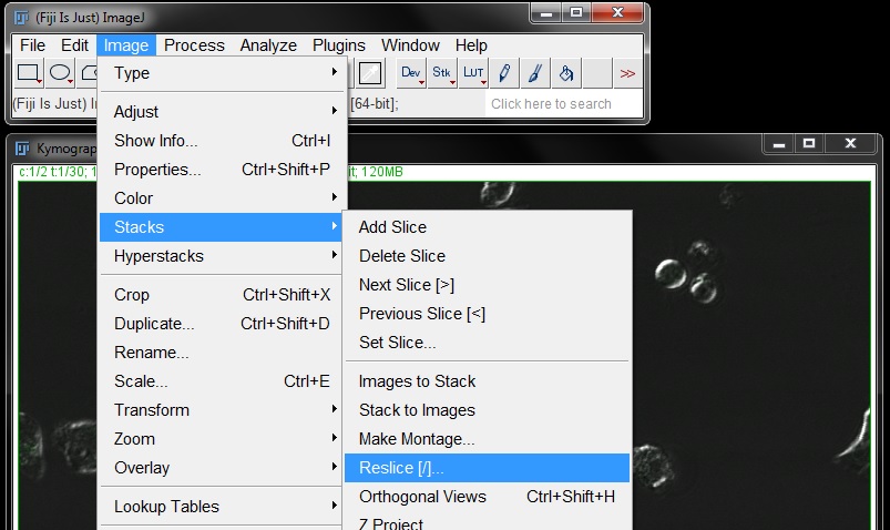
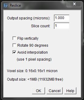
Go to Image -> Stacks -> Reslice and press OK in the resulting window.
The resulting image displays space on the x-axis, an intensity profile across the cells in brightfield and fluorescence. Time is displayed on the y-axis (top: start, bottom: end), you can see the green fluorescence intensity increase over time and the cell move left and right in the brightfield image.